Dieser Beitrag ist nur in englisch verfügbar

Introduction

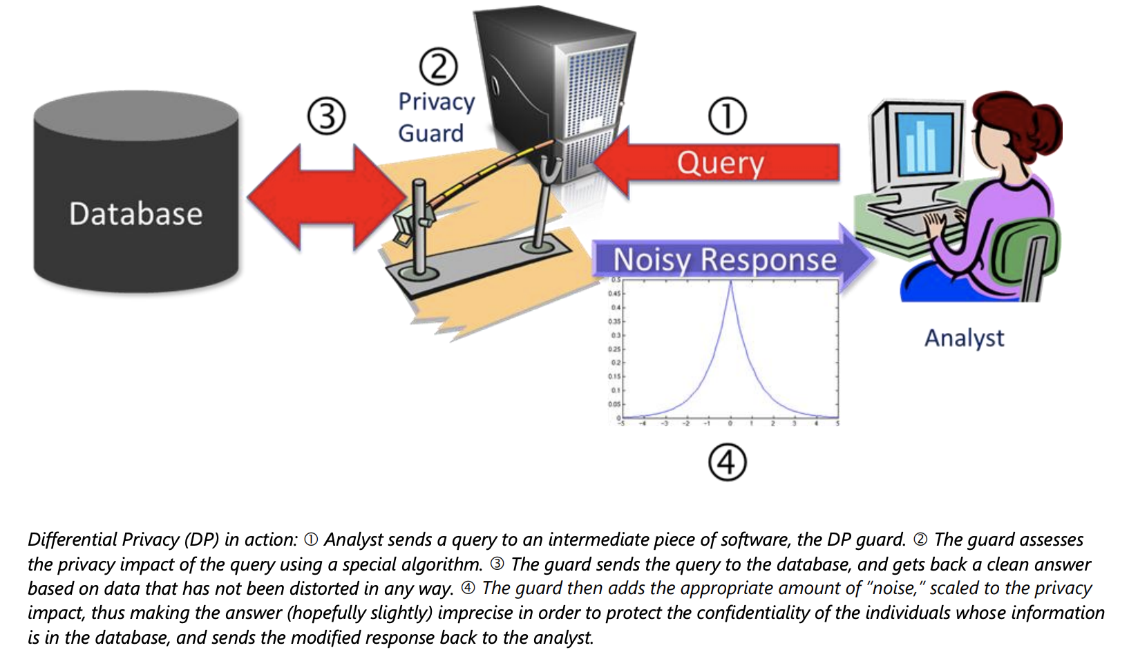
Differential privacy (DP) is nowadays considered the de facto standard for data protection. An intuitive explanation of DP is provided in our previous post. This post is instead aimed at readers who want to learn about the formulation of DP.

Let us assume we have a dataset D containing sensitive information about a group of people. In particular, each individual in the group is associated with a single data record containing her private information, for example her health status (Tab. 1).

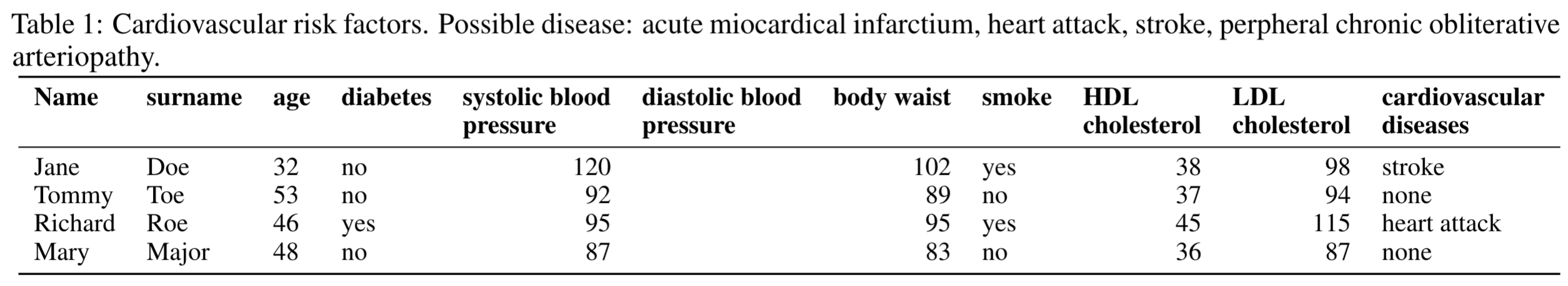
To help medical research on cardiovascular diseases, we would like to make the dataset publicly available, without however jeopardizing the privacy of the individuals in it. A privacy breach may happen because the information released inadvertently

1. discloses whether a person belongs to the group of people in D or not;
2. leaks private information about an individual of the group.

Below we show how DP prevents these privacy breaches.

The failure of privacy by anonymization

One may think that anonymizing the dataset D solves any privacy issue: each data record is processed so that any potential instance of personally identifiable information is removed: name, surname, address, fiscal code, etc. By deleting personal identifiers, the entire anonymized dataset can be published, so the logic. Both privacy risks 1 and 2 listed above seem to be prevented.

However, anonymization does not preserve the privacy of the data at all. Even worse, it generates the fatal illusion of achieving data protection when privacy is actually at severe risk. Indeed, combining information from the anonymised dataset with suitable additional data, sometimes even publicly available, can compromise the privacy of the dataset. And nowadays, in the epoch of big data, finding suitable additional data can be surprisingly easy… This happened, for example, in 2006, when Netflix released an anonymized dataset with 10 million movie rankings by 500,000 customers. It contained two to eight movie-ratings and dates of ratings for each anonymous customer. Netflix users were identified by matching their ratings and dates of rating with movie reviews and review timestamps from the public Internet Movie Database (in this database many users rank movies under their real names). The themes of rated movies may reveal private details about the users, like their own opinions on religion or ethical issues.

Combining information across datasets to achieve de-anonymization potentially works in many contexts other than the above Netflix case. For example, the massive amount of users’ queries in Google can be exploited to de-anonymize a commercial database with online purchases or de-anonymize health data containing searches of medical terms.

Privacy by randomization to the rescue

Because anonymous data is actually not so anonymous, the next best idea would be to only share information contained in D in the form of aggregate statistics. Our previous blog post however explained why even releasing plain aggregate statistics puts the privacy of the data at risk. A safer approach is to purposely inject a controlled amount of noise into the data and releasing the aggregate statistics on the noisy data rather than on the original ones. Our blog post explained how this approach protects the privacy of the data. In particular, noise was injected into the input values of the aggregate statistic f(D) to be computed, a method known as input perturbation. A different method, called output perturbation, consists of first computing the aggregate statistic f(D) on the original data and then perturbing f(D) by adding a noise value η drawn from a symmetric zero-mean probability distribution. The name output perturbation underlines that the output value of the data function f is perturbed, unlike input perturbation where the input values of f are perturbed. A pictorial explanation of output perturbation can be found in figure 1.

For both input and output perturbation, the logic remains the same: privacy by randomization. Generally, computing an aggregate statistic f(D) over the sensitive data D is a deterministic algorithm: if the statistic is re-computed, the same exact result is obtained. However, output- and input-perturbation methods are randomized algorithms. Running a randomized algorithm A multiple times on the same input will return different results each time. The output of A is therefore a random variable. Its mean is equal to f(D), since the noise values η are drawn from a symmetric zero-mean distribution.

To understand how randomization prevents leakage of sensitive information from private data, let us get back to our example: a private dataset D containing sensitive health information about a group of people (each user corresponds to a record), perturbed aggregate statistics about the data made publicly available. A malicious user, Luthor, wants to know whether a certain person belongs to the group, i.e., whether a certain record r exists in D or not. We can even pick the worst-case scenario: Luthor got to know all the records in D except r. Let D’ = D - {r}. If, in general, an aggregate statistic f(D) is released without being perturbed, Luthor can infer with certainty whether r is in D or not, by simply comparing f(D) with f(D’). However, if f(D) is perturbed before being released, this is no longer the case.

Let A(D) be the perturbed statistic obtained by applying a randomized algorithm A to the computation of f(D). For, example, in the case of output perturbation:

with η being sampled from a symmetric zero-mean distribution. In the remaining of this blog we will focus on output perturbation.

Calibrating the amount of noise

So far, we have seen how data privacy can be achieved by injecting noise into the output of the computation of f(D). But how much noise is needed to protect the data? Clearly, injecting too much noise renders the information contained in the data useless, since the difference between A(D) and f(D) gets arbitrarily large and thus the accuracy of A(D) decreases. We need to bound this difference. On the other hand, too little noise might reveal information about the data, putting privacy at risk. Indeed, if the magnitude of the noise is not height enough, Luthor can draw strong inferences about the data. For example, if repeated computations of A over D consistently generates values significantly smaller than f(D’), Luthor can be reasonably confident that r is not in D. Differential privacy basically quantifies the amount of noise needed in order to ensure the privacy of the data.

Differential privacy: mathematical guarantee of privacy

Let us consider a sensitive dataset D and any dataset D’ differing from D in exactly one record. That is, D’ may be: 1. a copy of D with one additional record, 2. a copy of D with a record removed, 3. a copy of D with the data in a single record changed (in this latter case, D and D’ have the same number of rows). Two datasets D and D’ differing in exactly one record are usually referred to as “neighbours”.

Differential privacy is a property of some randomized algorithms. Given a dataset D, a randomized algorithm A is ε-differentially private if, for any dataset D’ neighbour of D:

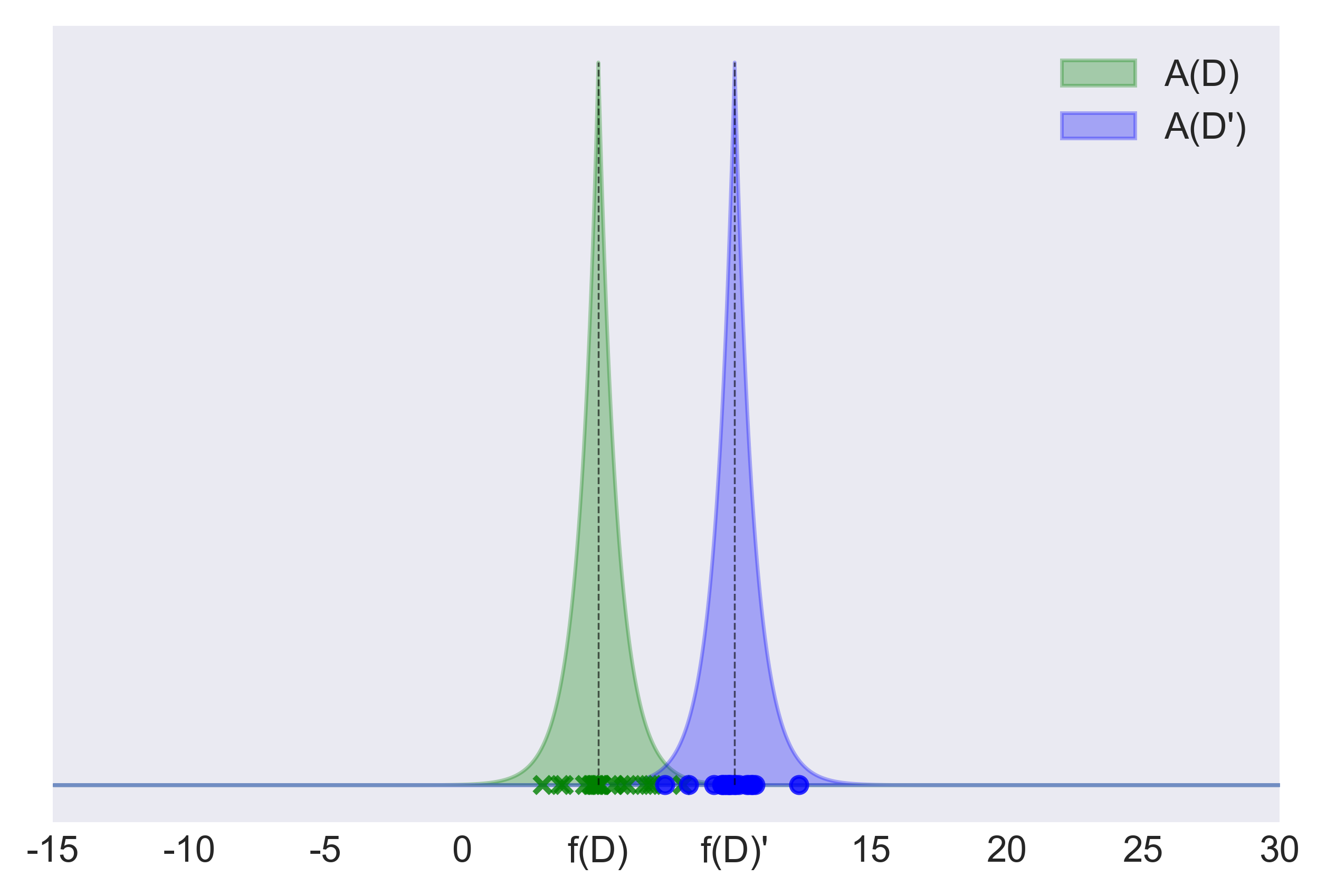
In other words, a differentially-private algorithm A guarantees that its output does not change significantly, as quantified by parameter ε, if any single record in D is removed or modified, or if a new record is inserted in D. This means that when observing the result a of a differentially-private algorithm A over a sensitive dataset D, Luthor cannot be confident that a certain record r is in D or not, since the probability that A returns a is nearly the same whether r is in D or not. A graphical explanation of Eq. (2) is provided by figure 2.

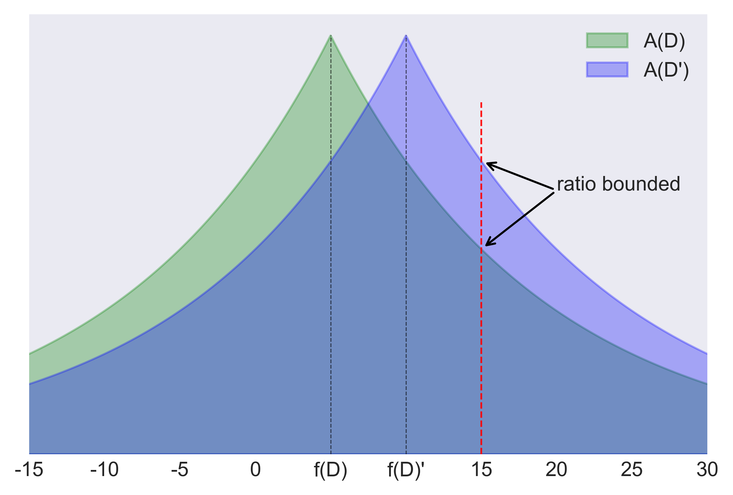
The parameter ε defines how close the probability distributions of the outputs of A on D and D′ must be, by bounding the ratios of their probabilities for every possible range of values which an output of A may fall in. In other words, ε specifies the privacy level of the differentially private algorithm A. The lower the value of epsilon is, the stronger the required privacy level is, since the bound on the probability ratios gets tighter, making the two probability distributions so similar that the likelihood of a certain value is almost the same under the two distributions.

After the seminal work introducing differential privacy, the adoption of more sophisticated metrics than the inequality in Eq. (2) to quantify the similarity between the distributions of the outputs of A(D) and A(D’) have been proposed in the literature. These metrics led to different formulations of DP, like, e.g., Rényi differential privacy. They might be an interesting topic for future blog posts, however in the following we focus on Eq. (2).

A closer look at the DP formulation

In order to fully understand Eq. (2), let us imagine that Luthor observes an arbitrary output a of a randomized algorithm A run on the actual dataset D. If a is much more likely to be generated when running A on D than it is when running A on another dataset D’ (differing from D in one record), observing a provides evidence that the actual database is D rather than D’. One may interpret this evidence as the privacy loss incurred when observing a. The privacy loss can be quantified as follows:

That is, the privacy loss is the log-ratio between the mass of a in the distribution of the outputs of A(D’) and mass of a in the distribution of the outputs of A(D). The log-ratio may be positive (when an event is more likely under D than under D’) or negative (when an event is more likely under D’ than under D). Differential privacy guarantees that the absolute values of the privacy loss is at most ε, for any possible output a that may be observed and any possible dataset D’. The ε parameter is often referred to as privacy loss parameter. When introducing Eq. (2) we called ε the privacy level. The two terms are used interchangeably in this post. We discuss plausible values for ε below, when we address the application of DP.

Back to noise calibration

We can now quantify the amount of noise needed by output perturbation (Eq. (1)) to satisfy the ε-differential privacy property, i.e., to achieve the privacy level defined by the ε value. Clearly, the amount of noise depends on the aggregate statistic f to be computed over D. In particular, the closer the values f(D) and f(D’) are, with D, D’ being neighbouring datasets, the lower the amount of required noise is. Therefore we might just calibrate the noise based on the neighbour D’ maximizing |f(D) - f(D’)|, to ensure protection even in the worst-case scenario. However, the amount of noise should not be calibrated based on the actual dataset D to be protected. Indeed, calibrating the noise based on D may disclose information about the data, since the amount of noise adopted would change across different datasets. To satisfy DP, the amount of noise is calibrated by considering all the possible datasets in the domain of interest. Given the set of all possible datasets, the sensitivity Δ(f) of a function f is defined as follows:

The amount of noise adopted in a differentially-private computation of f is proportional to the sensitivity of f. More sensitive functions requires more noise to ensure a certain privacy level. A widely-used approach to implement differentially private computations of f consists of sampling the noise value η in Eq. (1) from the Laplace distribution with location parameter zero and scale parameter Δ(f)/ϵ. This approach is commonly referred to as Laplace mechanism. For example, the green curve in figure 2 depicts the distribution of the output of the Laplace mechanism, applied to protect the value f(D) = 5 of a function f with sensitivity Δ(f)=7. The privacy level ε is arbitrarily set to 0.5.

With the Laplace mechanism, the (expected) error of the approximation A(D) of f(D) depends on the parameters of the Laplace distribution only, and not on the data D. Indeed, the variance of the Laplace distribution with location parameter zero and scale parameter Δ(f)/ϵ is equal to 2*(Δ(f)/ϵ)2 and, by definition, the variance is the expected value of the squared deviation from the mean.

The Laplace mechanism is the first implementation of DP. For our more curious readers, the choice of the Laplace distribution is basically what motivates the use of the exponential term exp(ε) in Eq. (2) rather than ε itself. The adoption of exp(ε) enables to follow the conventional interpretation of the ε symbol in mathematics, representing “a quantity as small as possible”. Indeed, when ε gets close to zero, exp(ε) converges to one, yielding stronger privacy levels. However, there is a more technical reason behind the choice of the exponential term exp(ε) : the “sliding” property of the Laplace distribution. If the location parameter of the Laplace distribution is shifted by one unit, the probability Pr(x) changes by a multiplicative factor up to exp(1). If the scale parameter is first multiplied by 1/ε, the multiplicative factor becomes exp(ε). This simplifies the proof of the Laplace mechanism.

Applying DP

To apply the Laplace mechanism for safely releasing the value of an aggregate statistic f, one needs to:

1. compute Δ(f);
2. set ϵ.

For example, if f is a plain count, e.g., counting the records satisfying a given property, its sensitivity is one. If f computes the mean of a column, its sensitivity depends on the range of possible values in the column. Indeed, it is equal to (ub - lb) / n, where [lb, ub] is the range of possible values and n the number of records. To define the range, one could be tempted of simply taking the minimum and maximum values of the column. However, this is not a good idea, since the resulting sensitivity would depend on the dataset D at hand, thus possibly leaking information about D. As matter of fact, in Eq. (3), the sensitivity is defined over all the possible datasets in the domain of interest: it does not depend on the D at hand. Therefore one should define plausible values for the lower and upper bound of the range by relying on her a priori knowledge of the domain only. For example, a reasonable range for an age column is 0 - 110 (apparently there are quite a few people older than 100 around the world…), regardless of the youngest and oldest person in D. On the other hand, it is also crucial to not over-estimate the range, for example by setting an age range to 0 - 300. Indeed, the larger the range is, the larger the sensitivity of the mean function is, yielding the Laplace mechanism to inject more noise, and thus decreasing the accuracy of the reported results. For the readers of our previous blog post, it should be now clear(er) how we defined the age range in the toy example that we used there.

Setting a range for an age column is relatively straightforward. But what about a reasonable range for the income of a group of people? Or for the price of houses? And for the number of km travelled in a year? Sensitivity is a rather complex topic, which would probably deserve a dedicated post. As you can see, applying DP is not really straightforward, different pitfalls need to be avoided.

Setting ε

When applying the Laplace mechanism, in addition to computing the sensitivity of a function, one also must set the ε value. Again, like bounding the range of possible values to compute Δ(f), setting ε is not always obvious.

Larger degrees of privacy cannot be obtained free of charge. Indeed, by the definition of the Laplace mechanism, a stronger privacy guarantee requires a larger amount of random noise. By consequence, the accuracy of the differentially-private estimations of an aggregate statistic decreases: stronger privacy is obtained at the cost of results accuracy.

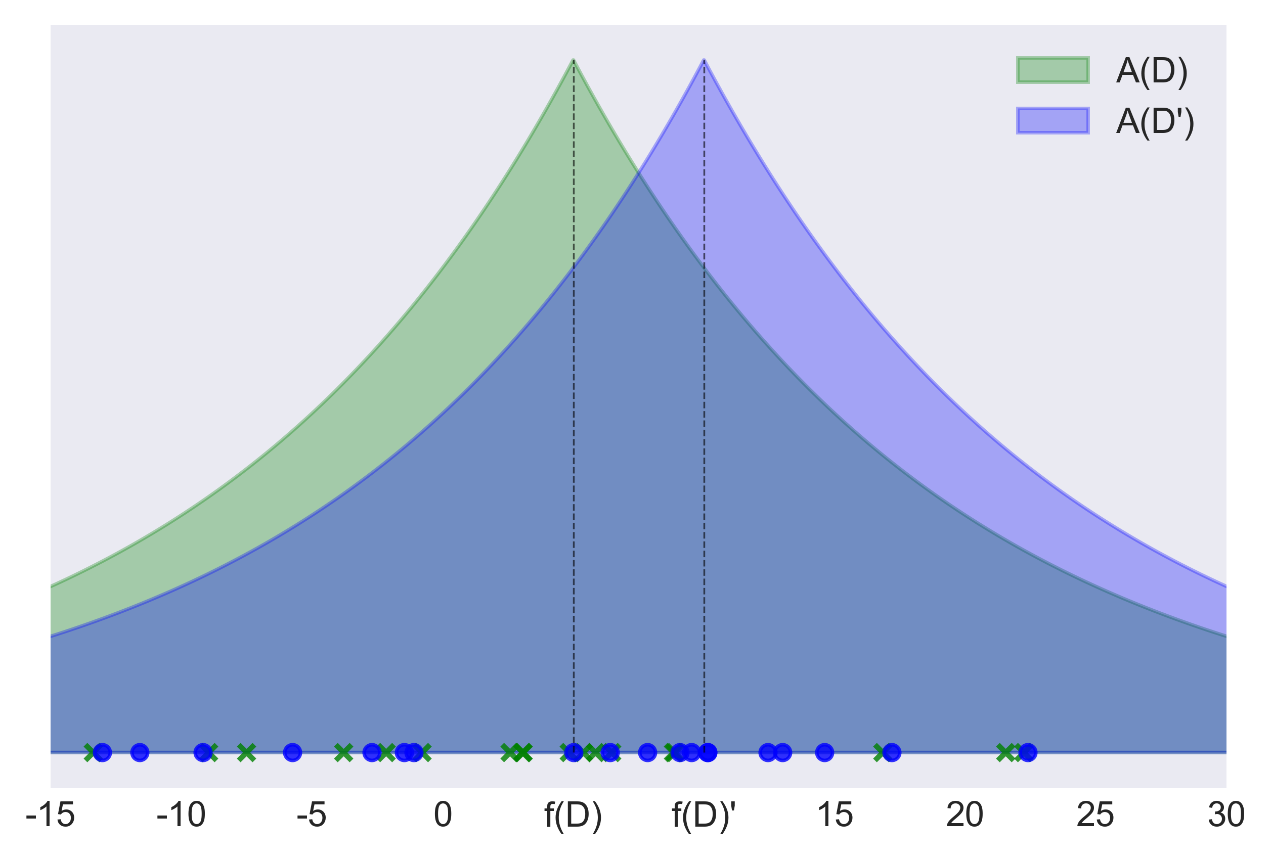
Even though ε can assume any non-negative value in ℝ, since it is exponentiated, values equal to 10 already allow Pr(A(D) ∈ S) to be around 22000 times larger than Pr(A(D’) ∈ S): this basically means no privacy at all. While, for example, with ε = 2, the bound on the probability ratio is 7.389. To get an intuition of what these values mean in practice, figure 3 and 4 depicts the scenarios observed when setting the privacy level ε to 0.5 and to 10, respectively.

Which value should we therefore set for ε, in order to avoid privacy leakage? This is still an open question in the DP community. Following the general consensus, it should be smaller than one, while values of above 10 are usually considered not useful to protect privacy. This is however just a rule of thumb and it might turn out to be excessively conservative.

Extra care is needed in setting epsilon when multiple differentially-private computations on the same dataset D are allowed. This is the topic of the remaining part of the post.

Repeated computations

One of the most elegant (and useful!) features of DP is the following one:

Basically, when running multiple ε-differentially private computations on the same dataset D, the overall privacy level decreases linearly in ε. This means that an increasing amount of sensitive information is leaked.

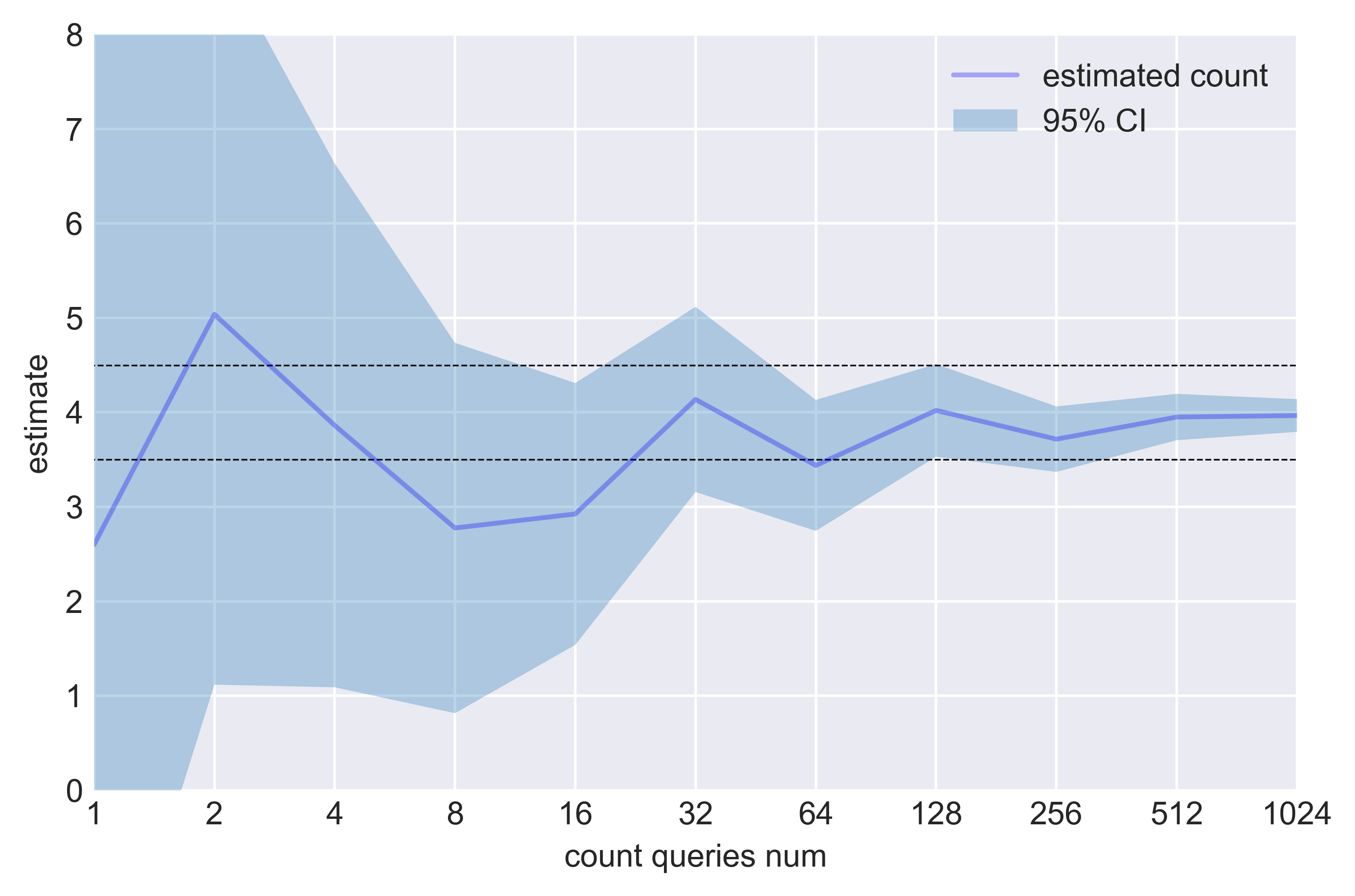
This is consistent with the intuition and with the law of large numbers in statistics. If the output perturbation mechanism in Eq. (1) is run multiple times, the noise injected to mask f(D) can be averaged out by taking the mean of the runs results A(D) observed. The larger the number of runs is, the better the approximation of f(D) obtained by taking the mean of the runs results is. This is empirically shown by figure 5, reporting the approximation of f(D) obtained across an increasing number of runs of a randomization algorithm A(D) implementing Eq. (1). Disclosing the actual value of an aggregate statistics f by averaging enough differentially-private estimations of f is usually known as averaging attack.

To control the cumulative privacy leakage across repeated computations of differentially-private mechanisms on the same dataset D, one may set a threshold εt on the overall privacy level. The threshold εt can be interpreted as privacy budget. The privacy budget defines the maximum leakage of sensitive information accepted for a certain dataset D. Performing an ε-differentially private computation consumes ε units of the privacy budget, the cumulative consumption of budget across multiple differentially-private computations is estimated by applying the composition theorem. Once the privacy budget is exhausted, any additional computation on D is forbidden. Properly setting the privacy budget thus protects, among others, from the averaging attack.

As you can imagine, the composition theorem turns out to be extremely useful when designing differentially-private deep-learning algorithms, that repeatedly access the dataset D during training. This topic is however beyond the scope of this post and it is left for future discussions.

Finally, a clarification on the terminology adopted. DP allows only a limited number of differentially-private analyses on a dataset. The limit is defined by the privacy budget εt. Since this post discusses DP mainly from a practical perspective, limiting the number of possible analyses is considered as a weakness. From a practical perspective, it actually is. However, this issue cannot be completely understood without considering also a different (perhaps more theoretical) perspective. The inability to run an unlimited number of analyses on a dataset is not just a limitation of DP, but it is basically a consequence of the “Fundamental Law of Information Recovery”, stating that answering enough queries with enough accuracy allows to completely reconstruct a dataset. A limited number of queries is basically the price to pay for enabling each query to return results with some utility and for not limiting a-priori what information each query can return. It is somehow similar to what happens in statistics, where enough samples from an unknown distribution p(x) enable to generate an empirical distribution reasonably close to p(x).

In general, any analysis on any data (be it raw data, anonymized data, pseudonymized data, synthetic data or any other form) reveals some information about the original data set. Otherwise the analysis would be useless anyway. Differential Privacy gives us the tools the measure and restrict this “information leakage”.

Conclusion

This post just scratches the surface of DP. DP is a powerful technique: it provides mathematical guarantee of privacy protection. By bounding the privacy loss generated by a differentially private analysis on the dataset, DP can guarantee that anyone seeing the result of the analysis basically makes the same inference about any individual’s private information, whether or not that individual’s private information is included in the dataset.

Applying DP is however not straightforward. Differential privacy affects accuracy, and the extent of this effect depends inversely on the privacy parameter ε. Achieving a reasonable tradeoff between accuracy and data privacy indeed depends on careful settings of the privacy budget and on different design choices, including bounding the range of values of the columns in the dataset. In addition, if multiple differentially-private analysis are performed, it might be useful to define the proportion of privacy budget dedicated to each of them.

Implementation of Differential Privacy therefore requires a holistic approach in which privacy and data protection is part of the design and development process and ideally is embeded in a secure and transparent platform for privacy-preserving analytics.

Alle Blog-Einträge