Setting Epsilon Considering Utility-Privacy Trade-off

TL;DR

We used Shokri’s shadow model membership inference attack [Shokri2015, Shokri2017] method to measure privacy leakage of differentially private models to address the utility-privacy trade-off question and assess limitations of the method. Figure 1 shows models trained with no DP are susceptible to a Shokri attack, while differentially private models with sufficient instances per class are secure. Additionally, “good” differentially private models trained on sufficient data with an epsilon of 1 retain good utility, >80% accuracy compared to no DP.

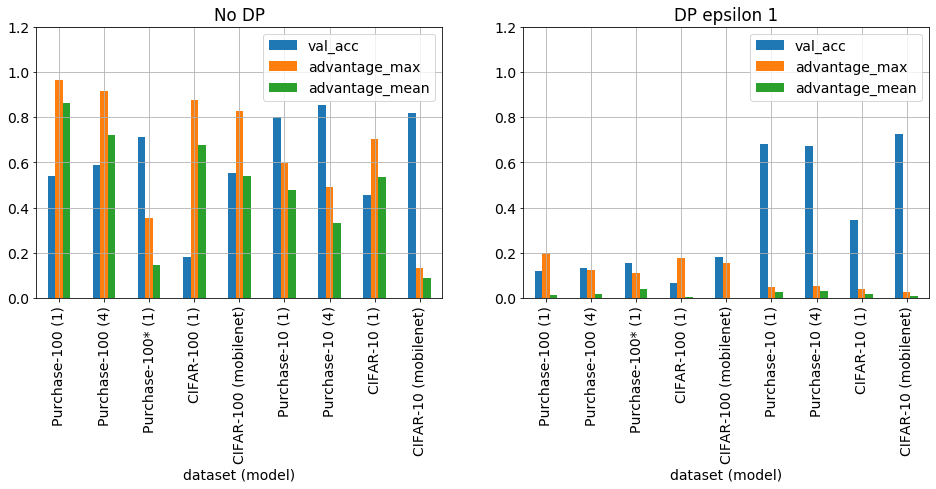
Figure 1. No DP and DP with epsilon 1, validation accuracy, maximum and average adversarial advantage of Purchase-100, CIFAR-100, Purchase-10 and CIFAR-10 trained on 10k instances for 100 epochs using different model complexities (see text for details). Purchase-100 was balanced using random oversampling and regularized training.*

Introduction

With the advent of General Data Protection Regulation (GDPR) and California Consumer Privacy Act (CCPA) and our increasingly data-driven society, there is an ever-growing demand for privacy preserving solutions for data utilization. Traditionally and contemporarily, non-disclosure agreements and different anonymisation techniques are used, though both suffer from deficiencies. The former is a contract of „trust”, with obvious problems, and the latter has suffered several significant failures, eg, AOL, Netflix, NY city taxi drivers and Australian Dep. of Health and releases data into the public domain, where the original data owner no longer has any control. Differential privacy has become a promising alternative.

Differential privacy (DP) is a strong, mathematical definition of privacy (eq. 1) in the context of statistical and machine learning analysis[Wood2019, Dwork2008]. In short, it returns noisy analysis results, where the amount of added noise inversely scales with the desired amount of privacy. What DP, or any other privacy preserving technique, cannot do is protect against publicly available information indirectly related to an individual. Let’s consider an example

Imagine Gertrude has a 100k€ life insurance policy with 1k€ premium or 1% of 100k€ based on her age and gender. Gertrude opts out of participating in a research study that finds women who drink coffee are more likely to suffer stroke. The insurance company decides Gertrude who drinks coffee now has 2% risk of dying and increase her premium to 2k€. This is the baseline case, where Gertrude already gave her details to the insurance company and study results were released with no direct connection to Gertrude, though still impacts her life.

Now imagine Gertrude participated in the study and the researchers conclude she has a 50% chance of dying from a stroke in the next year. If the results of the study were available to the insurance company, it might decide to increase her premium to 50k€. Fortunately, for Gertrude the researchers release a differentially private summary of the data with a DP guarantee of e = 0.01. In this case, the insurance companies estimate of Gertrude’s probability of dying next year could increase from 2% by at most 2% x (1 + 0.01) = 2.02% = posterior probability of dying due to participation = prior probability of opt out scenario x (1 + e).[adapted from Wood1029]

From above we have two neighbouring datasets D and D’ that differed by only one record, ie, the summary results with and without Gertrude’s record. The DP privacy guarantee e then bounds the variation in the output probabilities of a randomization function M() of D and D’, such that [Dwork2008, Jayaraman2019]:

Pr[M(D) ∈ S] < Pr[M(D’) ∈ S] x exp(e), (1)

where S is a set. The task of the randomization function M() is to add enough noise to an analysis to satisfy eq 1. The goal of a notional adversary is to use M() to differentiate between D and D’, representing a failure of privacy. The learner wants to extract useful statistics from D and D’ without violating privacy. Identifying a unique instance, that is the one that differentiated D from D’, such as Gertrude’s entry in the results, violates privacy. If the adversary can tell which set (D or D’) the learner is working on by the value of M(), then privacy is violated.[kdnugests]

The main challenge facing DP implementation is retaining data/model utility, while ensuring privacy. This utility-privacy trade-off is regulated by the privacy loss parameter e, which itself is derived from the parameters of the randomized function M(). Specifically, for a given epsilon, the required amount of randomization is dependent on the probability of identifying a single record, it then follows that this probability is dependent on the number of records and thereby inversely scales with size - think hiding in the crowd. Additionally, repeated passes over the dataset also change the probabilities – think repeated training loops.

To date, while the privacy guarantee bounded by e is mathematically well defined[Dwork2008], the practical implications regarding data leakage are not well understood. A recent paper systematically assessed the data leakage, as measured using three different attacks (2 variants of membership inference and 1 attribute inference attacks [Shokri2017, Yeom2018]) as a function of e for models DP-trained on two datasets CIFAR-100[ref] (images) and Purchase-100[ref] (structured data)[Jayaraman2019]. From a utility-privacy perspective, the results from Jayaraman2019 suggest that achieving acceptable utility and privacy is not possible in the given scenario.

It should be noted that the attacks referenced above and used in this report are all performed in a controlled environment, where the full training set is tested for leaks and the the required neighbouring (shadow) dataset is taken from the original dataset. Neither of these conditions reflect a real world scenario, where the adversary must first generate a shadow dataset (see Shokri etal 2017) and likely has a few instances they want to leak and with unknown classification label.

In this report, privacy leakage will be assessed using Shokri’s shadow model membership inference attack method [Shokri2015, Shokri2017] and a metric called adversarial advantage taken from Yeom etal [Yeom2018]. The leakage will be determined for different datasets (Purchase-10, Purchase-100, CIFAR-10 and CIFAR-100), model architectures and DP hyper-parameters. As this approach is applied in a controlled environment as described above a further real world attack on CIFAR-10 will be presented. The computational performance of DP training was characterized for different dataset and model properties. It will be shown that previous work [Jayaraman2019] has focused on datasets and models vulnerable to privacy leakage, resulting in low utility and privacy. In contrast when, datasets with reasonable properties and high performance models are employed, it is possible to attain both high utility and privacy, i.e, >80% utility compared to a model trained with no DP and near complete and complete privacy in the controlled environment and real world attack scenarios†, respectively.

† This based on synthetic data generation method. It would be cool to get images, e.g, from google, and make them CIFAR format then try again.

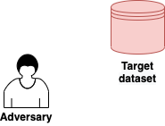
Figure 2. Place holder for flow diagram of attacks in controlled and real world settings.

Method

Datasets

The datasets used in the attacks were Purchase-10, Purchase-100, CIFAR-10 and CIFAR-100.

Purchases are derived from Kaggle's Acquire Valued Shoppers Challenge [https://www.kaggle.com/c/acquire-valued-shoppers-challenge/data] transactions.csv data. This file contains a minimum of 1 years worth of purchases for over 300 k shoppers. To create the Purchase datasets, a list of the first 600 items is created and then a new dataset of customers and 600 binary features indicating if they ever purchased this item is created. Finally, this derived dataset is clustered using knn to provide 10 or 100 class labels. Add oversampling details.

CIFAR-10 and 100 are balanced benchmark datasets of 60 k colour images of 32 x 32 pixels of 10 and 100 classes, respectively. For the attacks the 50 k training and 10 k test images were combined to create 1 dataset. For the simple Neural Network model an additional preprocessing step was performed using principle component analysis (PCA) to extract the first 100 (increased from 50 as in Jayaraman2019) principle components.

Attacks

Attacks were performed using Keras version 2.3.1, TensorFlow 1.15.2, TensorFlow-Privacy 0.2.2, TensorFlow Hub 0.7.0 and python 3.7.5 on an Azure Standard D32ds_v4 (32 vcpus, 128 GiB memory) running linux server 18.04-LTS.

Target models

Target models were trained using an Adam or VectorizedDPAdam optimizer with learning rate of 0.001 and batch size of 100. The DP models were trained using nominal epsilon values of 0.01, 0.1, 1, 10, 100, and 1000 [footnote], l2_norm_clip of 1 and num_microbatches equal to the batch size of 100. The training and test sets were 10k each unless otherwise indicated.

The target models used for Purchase were neural networks with 1 dense layer of 128 nodes, tanh activation, plus a softmax and L2 regularization of 1e-8 trained for 15 and 100 epochs.

The simpler target model for CIFAR used the 100 PCA feature dataset and a neural network of 1 layer with 512 modes, tanh activation, plus a softmax and L2 regularization of 1e-3 trained for 40 and 100 epochs with learning rate 0.001, and batch size 100. A more complex model used a tensorflow hub mobilenet_v2_035_96 [link/footnote] version 4 transformer with frozen weights followed by a dropout of 0.5 and a softmax with L2 regularization of 1e-8. The original 32 x 32 images were resized using tf.image.resize to the full 96 x 96 pixel input of the transformer. The model was trained for 10 and 100 epochs.

Shadow Models

20 shadow models plus 1 validation shadow model were trained on 10 k training and 10k test data randomly selected from the remaining samples after the target dataset was sampled. The shadow model architecture and parameters were the same as the corresponding target model.

Attack datasets

An attack dataset is created by taking a trained model, target or shadow, and predicting on the train and test datasets to retrieve the probabilities, which become the attack dataset features and the labels are 1 for training and 0 for test. Additionally, the original class label was also stored to enable per class attack model training.

Three attack datasets were created for each attack. An attack training set created from each of the 20 shadow models resulting in 400 k training instances, an attack validation set created from the validation shadow model and the third being the target attack dataset, which uses the target model used to test the actual leakage. This final dataset is artificial in the sense that it contains the information the adversary wishes to learn but does not possess.

Attack model

The same attack model was used for all attacks. It consisted of a single dense layer of 64 nodes, relu activation, L2 regularization of 1e-8 trained for 20 epochs with a batch size of 10. Separate attack models were trained for each of the original classes and 3 replicate attack model trainings were performed for each attack.

Metrics

Utility is measured using the target model test set accuracy and attack performance is characterized by precision and recall and adversarial advantage taken from Jayaraman etal 2019. It is defined as:

advantage = tp / (tp + fn) - fp / (fp + tn),

where tp, fp, fn, tn are true positive, false positive, false negative, true negative of the target attack dataset, respectively. Adversarial advantage has range -1 to 1, where values > 0 indicate there are more true positives than false positive, e.g., an advantage of 0.5 corresponds to 1.5 times more true positives than false positives. Note precision has a threshold value of 0.5 before an attack becomes successful, i.e., more true positives than false positives. These metrics are calculated for the entire and per target class of the training attack dataset and averaged over the three replicates. Precision and advantage are quoted as the maximum value for a single class, unless otherwise stated. Test accuracy is quoted as that determined for the final epoch.

Target model query shadow data generation

Synthetic data generation for CIFAR-10 and the MobileNet model followed the algorithm defined by Shokri etal 2017 with the addition of resizing the synthetic “image” from 32 x 32 pixels to 96 x 96 pixels before prediction. See discussion for parameterization.

Synthetic data generation

Synthetic data was generated using scikit-learn 0.23.1 make_classification function.

Results and Discussion

In the following, precision and advantage are quoted as the maximum value for a single class and test accuracy as determined at the final epoch.

Validation of Attack Procedure

Purchase-100

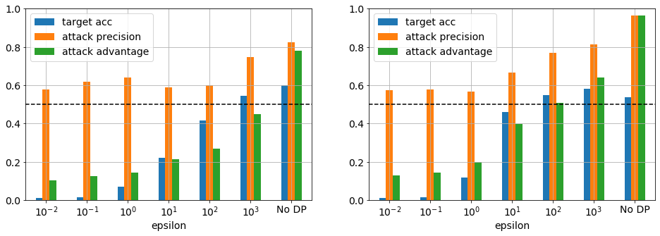
Figure 3. Target model accuracy and attack precision and advantage for Purchase-100 trained using a model with 1 layer for 15 (left) and 100 (right) epochs. At 15 epochs the target model validation accuracy was approximately maximum for no DP. The threshold precision before an attack is successful is 0.5 as indicated by the dashed line.

Figure 3 shows the target model test accuracy, attack precision and adversarial advantage for the Purchase-100 dataset as a function of DP epsilon, training epochs and model complexity. The no DP test accuracy at 100 epochs and 1 layer is 0.54, which results in a generalization gap of 0.46 as the train accuracy was 1 (not shown). The corresponding attack precision of 0.97 is comparable to previous studies [Shokri2017, Jayaraman2019]. At this point it is important to point out that this neither a good dataset nor model in terms of performance. The dataset has unbalanced classes and is small (10 k) compared the number of classes (100); the model is overfit and has no regularization to aid generalization resulting in low test accuracy and an extraordinarily high adversarial advantage. That said, if the model is now train from the perspective of a learner, one who wished to achieve high test accuracy, simply lowering the the number training epochs immediately increases the test accuracy (0.6 cpt 0.54) and lowers the adversarial advantage (0.97 cpt 0.78) for in the absence of DP.

Upon applying DP to the training, it can be seen that there is a significant reduction in both test accuracy and adversarial advantage as epsilon is decreased to the point where the model becomes essentially useless and nonetheless still leaks, i.e., advantage remains around 0.1. This results is consistent with Jayaraman etal 2019. In this configuration, DP simply cannot prevent leakage. Naively, one would assume that this is a result of the minority classes having too few instances; however, figure 4 shows this is not the case. The minimum class size is 11 instances and the classes with maximum adversarial advantage have > 80 instances. It is unclear what makes these classes more vulnerable to attack and requires further investigation.

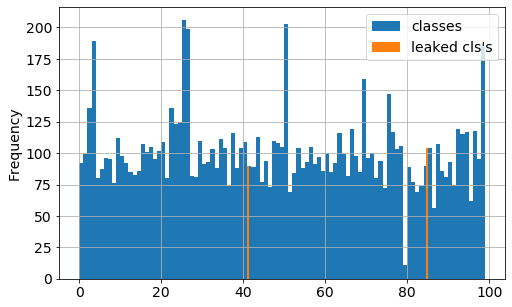
Figure 4. Purchase-100 train set probability distribution (blue) and classes with maximum adversarial advantage (orange). See which classes leaked in regulated and balanced training below.

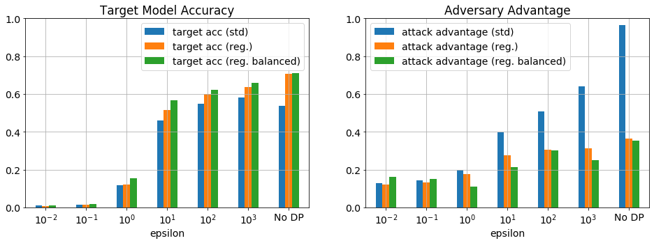
Figure 5. Comparison of attacks on Purchase-100 varying L2 regularization and balancing the dataset. The target model accuracy moderately improved with regularization and balancing; however, the attack performance was significantly reduced for epsilon greater than 0.1. The most successful attack from figure 3 was used, where the target model had 1 layer with 128 nodes and trained for 100 epochs. The L2 regularization was varied from 1e-8 (std) to 5e-3 (reg.) and the dataset was balanced using random oversampling (reg. balanced).

Again approaching the task from a learners perspective, figure 5 shows the effect of optimizing L2 regularization of the model and balancing the classes using oversampling. There is a clear improvement in the test accuracy and and the adversarial advantage for epsilon > 0.1, though this dataset and model remain susceptible to attack. Interestingly, the balancing of the classes has less of an effect than regularization, which is consistent with minority classes not being the largest leakers. Further optimization of training set size, the model size and the number of epochs would further improve this situation.

CIFAR-100

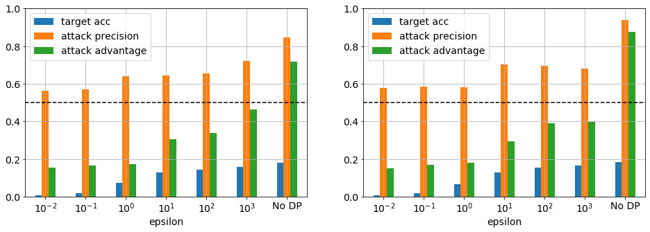
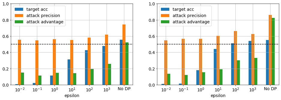
Figure 6. CIFAR-100 (top) trained on first 100 PCA features and a network with 1 layer, 512 nodes, tanh activation, and 1e-3 L2 regularisation for 40 (left) and 100 (right) epochs. (bottom) trained using MobileNet_96 feature extractor, dropout of 0.5 and softmax as target model for 10 (left) and 100 (right) epochs.

Continuing the validation of the attack method in this report, CIFAR-100 was also investigated. Figure 6 top right panel shows that using a similar dataset and model configuration as Jayaraman etal results in poor model and attack performance, achieving test accuracy 0.18 and advantage 0.88. Furthermore, in the presence DP training, leakage remains a problem regardless of epsilon. As was the case for Purchase-100, this dataset and model combination is optimized for privacy vulnerability, though highlights one of limits of DP in that too few instances per class (100 in this case) results in poor performance.

In an effort to improve performance, a more complex model including a MobileNet transformer was investigated (fig. 6 bottom row). As expected the model accuracy significantly improved but the adversarial advantage remained high, though significantly reduced. This is likely due to the small train set size, which is addressed in the next section.

To finish, the above serves as a validation of the attack method in this report and highlights that poor performing models in the absence of DP remain poor when DP is applied. These models would not be used in any real world scenario and thus remain firmly rooted in the domain of researching data privacy leakage and not the practical application of privacy preserving techniques.

More Instances per Class

Purchase-10

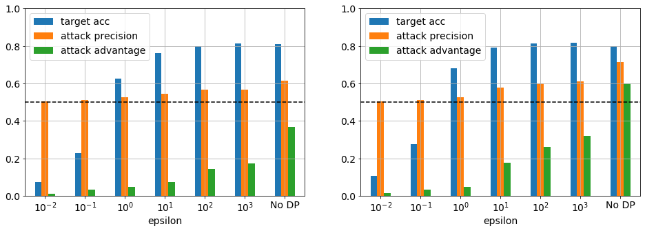
Figure 7. Target model accuracy and attack precision and advantage for Purchase-10 using the same parameters from figure 3 for a target model with 1 layer trained for 15 (left) and 100 epochs (right). There is a significant improvement in target model accuracy and reduction in attack performance compared to Purchase-100.

A look at figure 7 immediately shows that increasing the number of instances per class significantly improves model performance in both accuracy and privacy preservation. The former being of no surprise as is often the case with machine learning, more data is better [find references]. Generally, the accuracy remains high for epsilon ≥ 1 in contrast to the above results. Concentrating on the results for epsilon of 1, the test accuracy relative to no DP decrease from 0.81 to 0.63 and 0.80 to 0.68 (~18% loss) and the advantage from 0.37 to 0.05 and 0.60 to 0.05 for 15 and 100 epochs, respectively. The implications for an advantage of 0.05 are unclear, in particular if we look at the variation over the replicate attack model training we see the value is 0.050 with 95% CI [0.026, 0.074] for class 0 and 15 epochs and moreover the mean advantage over the complete target attack dataset is 0.019 with 95% CI [0.001, 0.037], which is starting to look like noise. Thus, an adversary with only a few instances with a target class not in the most vulnerable class would have no confidence in this attack.

CIFAR-10

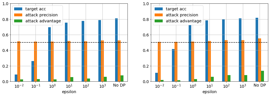
Figure 8. CIFAR-10 trained using MobileNet_96 feature extractor, dropout of 0.5 and softmax as target model for 10 (left) and 100 (right) epochs. The no DP model already exhibits good accuracy and relative low advantage. The DP models with epsilon > 0.1 retain the accuracy and lower the attack advantage.

The situation further improves for a balanced dataset with sufficient data and a more realistic model. Figure 8 shows the results for CIFAR-10 with a 1000 instances per class. The first observation is even in the case of no DP the adversarial advantage is low. This was likely aided by the addition of a dropout layer that is itself necessary to achieve high test accuracy or to phrase it differently, good generlization. Here the generalization gap is 0 for both epochs. Again, it can be seen the test accuracy remains high for epsilon ≥ 1. Focussing on epsilon 1, the test accuracy relative to no DP decreases from 0.81 to 0.70 and 0.82 to 0.72 for 40 and 100 epochs respectively. This corresponds to approximately 12 % loss of accuracy. The corresponding maximum advantage for class 4 is 0.025 with 95% CI [0.007, 0.043] and 0.028 with 95% CI [0.024, 0.032] for 40 and 100 epochs, respectively. As above, to complete the picture one needs to look at the mean advantage over the full target attack dataset, which is 0.004 with 95% CI [0.000, 0.006] and 0.009 with 95% CI [0.007, 0.011] for 40 and 100 epochs, respectively. Interestingly, the advantage for epsilon values > 1 exhibit good privacy and could be considered for a practical application.

Results Summary

Figure 9. No DP and DP with epsilon 1, validation accuracy, maximum and average adversarial advantage of Purchase-100, CIFAR-100, Purchase-10 and CIFAR-10 trained on 10k instances for 100 epochs using different model complexities (see text for details). Purchase-100 was balanced using random oversampling and regularized training.*

Figure 9 summarizes the complete set of attacks performed in this section. It is clear that Purchase-100 and CIFAR-100 trained on 10 k samples with simple models are vulnerable to privacy leakage. These are favourites of the literature [long list of papers] investigating privacy leakage. Furthermore, Jayaraman etal have based their entire work on these 2 datasets and concluded that DP was not practical to protect privacy because model utility could not be preserved. In stark contrast, in this report it was shown that more realistic datasets with on average a 1000 instances per class combined with useful models that actually generalize well and thereby achieve high test accuracy, trained for an optimal number of epochs can retain better than 80 % utility compared to the no DP counterpart and near complete privacy.

Real World Attack

To bring the discussion closer to reality a “real world attack” was performed on CIFAR-10 using the MobileNet model and epsilon 1 (~70% accuracy), though trained on the entire dataset (all 60 k), as would occur in the real world after initial development was completed. Thus an adversary would be left with the problem of how to acquire shadow model training data. A synthetic data generation process was proposed by Shokri etal 2017, which queries the target model for each target class until the synthetic data meets minimum criteria of probability and correctly classifying the class [Shokri2017]. This process is repeated until a sufficient number of instances has been created. This method was employed using the same parameters as Shokri etal 2017 with the exception of the minimum probability being set to either 0.5 or 0.9 over two experimental runs. In both cases the resultant probability distribution per class were narrow and near the minimum probability. Upon training the shadow models it became clear that with such narrow probability distribution there was no possibility for the model to differentiate between train and test sets. Evaluation on the shadow validation set confirmed this finding. Thus, using this method it was not possible to attack this model and dataset. This is in contrast to the results of Shokri etal who attacked the Purchase dataset (assumed 100 based on performance), where there were 600 binary features. As known from here and others[refs], Purchase-100 is a particularly vulnerable dataset and one only needs to vary features from 0 or 1, whereas for CIFAR the 3072 features are continuous between 0 and 1. Moreover, Shokri etal attacked a model trained without DP, whereas the DP trained model here should, as evidenced from the results in figure 8 make the predicted probabilities private in nature, thus rendering the synthetic data generation process unusable.

Effect of l2_norm_clip

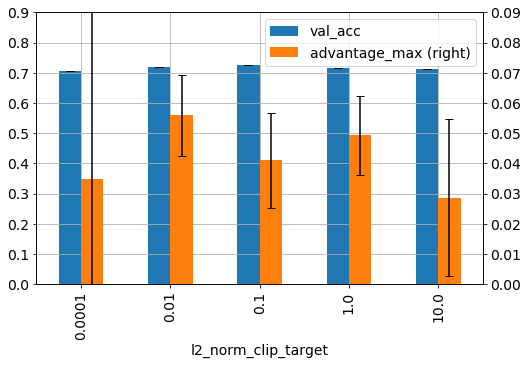
Figure 10. CIFAR-10 trained as above for MobileNet with epsilon 1 and varying l2_norm_clip and for 80 epochs.

Figure 10 shows the effect of l2_norm_clip on model accuracy and adversarial advantage for CIFAR-10 trained on the MobileNet model with epsilon 1. There is little effect on the model accuracy and as this was trained only once per l2_norm_clip value cannot be assess beyond natural model variation. The adversarial advantage (right axis), does show some l2_norm_clip dependence. The advantage is lowest for the highest value of 10 and highest for a low value of 0.01. The advantage at 0.1 and 1 are intermediate from these to values and not significantly different. This is the expected outcome, as the amount of noise added during DP learning is bounded by l2_norm_clip of the gradients, thus when 2_norm_clip is high more noise is added and vis versa. The outlier l2_norm_value of 0.0001 shows how unstable the learning can become with the error bars of the advantage extending beyond the y-axis limits and thus extreme values of l2_norm_clip are not recommended. That said, a small study using the mnist tutorial from TensorFlow-Privacy on Colab showed that when varying the number of microbatches, l2_norm_clip becomes an important parameter to achieve high accuracy.

DP Computation time

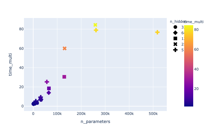
Figure 11. computation time multiplier (DP/noDP) for DP versus non-DP for different number of features and nodes in a single layer network.

Using synthetic data with 10 classes and 50 k instances, 10, 50, 100, 500 and 1000 features, trained on a network with 1 layer and 32, 64, 128, 256 and 512 nodes for 1 epoch, the time for no DP and DP training was determined. Figure 11 shows the increase in training time for DP compared to no DP, calculated as DP/no DP. It is clear that as the number of model parameters increases the DP training time increases until reaching saturation at 80 x longer near 250 k parameters. This is due to the need to calculate the per instance gradient (when num_microbatches = batch_size) to allow gradient clipping. It is possible to improve the computation time by decreasing the number of microbatches but this comes at the expense of accuracy and for many datasets this cost is too high (not shown).

The problem increases when convolutional layers are added. Using CIFAR-10 on 50 k samples with 2 convolutional layers with maxpooling resulting in 37,274 trainable parameters it takes ~100 times longer to train DP compare to no DP. The corresponding model with no convolution or maxpooling and ~100 k parameters takes only ~16 time longer. There is currently no explanation for this phenomena.

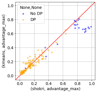
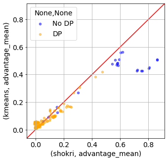
Figure 12. Estimation of attack metrics advantage_max (left) and advantage_mean (right) using kmeans to separate the target model train and test probabilities into 2 clusters. The results are compared to the shadow model membership inference attacks (shokri).

Any data owner that wishes to protect their data but make it accessible will need the ability to estimate the practical leakage of the dataset and, as discussed above, combined with the desired target model. As shown in the previous section, the computation time of DP models can be quite high and combined with the need to train many shadow models can result hours of computation. Thus, while using shadow model membership inference attacks to estimate practical leakage is thorough it is not very efficient.

Figure 12 shows the comparison between the shadow model membership inference attack (shokri) results from above and those obtained using kmeans to cluster the target model train test probabilities. The kmeans results agree well with shokri with the exception of the target model being trained with no DP and very high leakage values. This is encouraging because the main use case of this method is to determine the leakage when DP is applied and ideally focused on lower values of these metrics, where the correlation is high. Moreover, figure S? shows the computation time for the kmeans (of order seconds) clustering is significantly faster than the corresponding time to compute 20 shadow models (minutes to hours). Thus this method can be used by a data owner, not only to quantify practical leakage but also to select an appropriate epsilon.

Summary

In this report, the results of membership inference attacks using the shadow model attack method proposed by Shokri etal to measure practical privacy leakage, quantified by adversarial advantage, of neural network models trained both with and without differential privacy on 4 different datasets: Purchase-10, Purchase-100, CIFAR-10 and CIFAR-100. In the first part, the attacks were validated using the same or similar approaches as Shokri etal and Jayaraman etal, where the results were shown to be consistent with these two studies. Specifically for Purchase-100 and CIFAR-100 with 10 k training instances, it was shown that it is not possible to protect the privacy of the 2 datasets using differential privacy consistent with the findings of Jayaraman etal. However, this was attributed to the low number of training instances and as evidenced by the second part. In the second part, it was shown using Purchase-10 and CIFAR-10 that differential privacy can not only reduce the adversarial advantage to near complete privacy but retain greater than 80 % of the accuracy compared to the model trained without any privacy protection. The former suggests that a dataset with an average of 100 instances per target class is insufficient to guarantee privacy, while in the second part 1000 instances suffices. Further investigation is required to determine a lower limit for the number of instances per class given different dataset properties, model generalizability and performance.

Notwithstanding the good results obtained under controlled conditions, it was shown for CIFAR-10 trained using differential privacy on the entire dataset and shadow data generated using Shokri etal’s model query synthetic data generation technique that it was not possible to leak any private information. This result is only relevant for the case where the adversary does not have access to a shadow dataset, which itself is not necessarily as realistic situation as to use the model means one has access to data. This experiment would be improved by generating shadow data from images sourced elsewhere.

Finally, in a real world setting and in general, if a learner wishes to train a model with high predictive power for new unseen data that model must have sufficient training data, generalize well and not be overfitted. This is true for any model, regardless of whether privacy preserving techniques are used. The above model properties are not well represent in literature related to membership inference attacks or privacy leakage when differential privacy is applied [shokri, jayaraman, ++]. In this context, the results of this report have shown, high performance models trained with differential privacy can retain both high utility and privacy.